Higher-Order Derivatives: Maxima and Minima

Review Exercises for Chapter 3

Question 3.156

Let $f$ be any differentiable function. Show that $u=f(y-kx)$ is a solution to the partial differential equation $\displaystyle \frac{\partial u}{\partial x} + k\frac{\partial u}{\partial y}=0$.

Question 3.157

Prove that if $u$ and $v$ have continuous mixed second partial derivatives and satisfy the Cauchy–Riemann equations \begin{eqnarray*} \frac{\partial u}{\partial x} &=&\frac{\partial v}{\partial y} \\[6pt] \frac{\partial u}{\partial y} &=&-\frac{\partial v}{\partial x}, \end{eqnarray*} then both $u$ and $v$ are harmonic.

Question 3.158

Let $f(x, y)=x^2-y^2-xy+5$. Find all critical points of $f$ and determine whether they are local minima, local maxima, or saddle points.

Question 3.159

Find the absolute minimum and maximum values of the function $f(x, y)=x^2+3xy+y^2+5$ on the unit disc $D=\{(x, y) \mid x^2+y^2 \leq 1\}$.

Question 3.160

Find the second-order Taylor polynomial for $f(x, y)=y^2e^{-x^2}$ at (1, 1).

Question 3.161

Let $f(x, y)=ax^2+bxy+cy^2$.

(a) Find $g(x, y)$, the second-order Taylor approximation to $f$ at (0, 0).
(b) What is the relationship between $g$ and $f$?
(c) Prove that $R_2(\textbf{x}_0, \textbf{h}) = 0$ for all $\textbf{x}_0, \ \textbf{h} \in \mathbb{R}^2$. (HINT: Show that $f$ is equal to its second-order Taylor approximation at every point.)

Question 3.162

Analyze the behavior of the following functions at the indicated points. [Your answer in part (b) may depend on the constant $C$.]

(a) $z = x^2 -y^2 + 3xy, \qquad (x,y)= (0,0)$
(b) $z = x^2 -y^2 + Cxy, \qquad (x,y)= (0,0)$

Question 3.163

Find and classify the extreme values (if any) of the functions on ${\mathbb R}^2$ defined by the following expressions:

(a) $y^2 - x^3$
(b) $(x -1)^2 + (x-y)^2$
(c) $x^2 +xy^2 + y^4$

Question 3.164

(a) Find the minimum distance from the origin in ${\mathbb R}^3$ to the surface $z = \sqrt{x^2 -1}$.
(b) Repeat part (a) for the surface $z= 6xy +7$.

212

Question 3.165

Find the first few terms in the Taylor expansion of $f(x,y)= e^{xy} \cos x$ about $x=0$, $y=0$.

Question 3.166

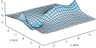
Prove that \[ z=\frac{3x^4-4x^3-12x^2+18}{12(1+4y^2)} \] has one local maximum, one local minimum, and one saddle point. (The graph is shown in Figure 3.24.)

Figure 3.24: Graph of $z= \hbox{(}3x^4-4x^3-12x^2+18\hbox{)}/12\hbox{(}1+4y^2\hbox{)}$.

Question 3.167

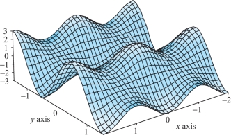
Find the maxima, minima, and saddles of the function $z=(2+\cos\pi x)(\sin \pi y)$, which is graphed in Figure 3.25.

Figure 3.25: Graph of $z= \hbox{(}2+\cos\pi x\hbox{)}$ $\hbox{(}\sin \pi y\hbox{)}$.

Question 3.168

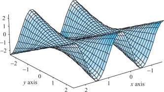
Find and describe the critical points of $f(x,y)=y\sin\,(\pi x)\,$. (See Figure 3.26.)

Figure 3.26: Graph of $z=y\sin\hbox{(}\pi x\hbox{)}$.

Question 3.169

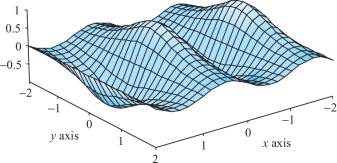
A graph of the function $z=\sin(\pi x)/(1+y^2)$ is shown in Figure 3.27. Verify that this function has alternating maxima and minima on the $x$ axis, with no other critical points.

Figure 3.27: Graph of $z=\sin\hbox{(}\pi x\hbox{)}/\hbox{(}1+y^2\hbox{)}$.

In Exercises 15 to 20, find the extrema of the given functions subject to the given constraints.

Question 3.170

$f(x,y)=x^2-2xy+2y^2$, subject to $x^2+y^2=1$

Question 3.171

$f(x,y)=xy-y^2$, subject to $x^2+y^2=1$

Question 3.172

$f(x,y)=\cos(x^2-y^2)$, subject to $x^2+y^2=1$

Question 3.173

$f(x,y)=\displaystyle \frac{x^2-y^2}{x^2+y^2}$, subject to $x+y=1$

Question 3.174

$z=xy$, subject to the condition $x+y = 1$

Question 3.175

$z = \cos^2 x + \cos^2 y$, subject to the condition $x+y = \pi/4$

Question 3.176

Find the points on the surface $z^2- xy = 1$ nearest to the origin.

Question 3.177

Use the implicit function theorem to compute $dy/dx$ for

(a) $x/y =10$
(b) $x^3 - \sin y + y^4 = 4$
(c) $e^{x + y^2} + y^3 =0$

213

Question 3.178

Find the shortest distance from the point $(0, b)$ to the parabola $x^2-4y = 0$. Solve this problem using the Lagrange multiplier method and also without using Lagrange’s method.

Question 3.179

Determine all values of $k$ for which the function $g(x, y, z)=x^2+kxy+kxz+ky^2+kz^2$ has a local minimum at $(0, 0, 0)$.

Question 3.180

Find and classify all critical points of the function $g(x, y)=\frac{1}{4}x^4-\frac{5}{3}x^3+y^3+3x^2-\frac{3}{2}y^2+20$.

Question 3.181

Solve the following geometric problems by Lagrange’s method.

(a) Find the shortest distance from the point $(a_1,a_2,a_3)$ in ${\mathbb R}^3$ to the plane whose equation is given by $b_1 x_1 +b_2 x_2 + b_3 x_3 +b_0 = 0$, where $(b_1,b_2,b_3)\neq (0,0,0).$
(b) Find the point on the line of intersection of the two planes $a_1 x_1 +a_2 x_2 + a_3 x_3 = 0$ and $b_1 x_1 +b_2 x_2 + b_3 x_3 +b_0 = 0$ that is nearest to the origin.
(c) Show that the volume of the largest rectangular parallelepiped that can be inscribed in the ellipsoid \[ \frac{x^2}{a^2} +\frac{y^2}{b^2} +\frac{z^2}{c^2} =1 \] is $8abc/3\sqrt{3}$.

Question 3.182

A particle moves in a potential $V(x,y)= x^3 - y^2 + x^2 + 3xy$. Determine whether (0, 0) is a stable equilibrium point; that is, whether or not $(0,0)$ is a strict local minimum of $V$.

Question 3.183

Study the nature of the function $f(x,y)=x^3 - 3xy^2$ near (0, 0). Show that the point (0, 0) is a degenerate critical point; that is, $D=0$. This surface is called a monkey saddle.

Question 3.184

Find the maximum of $f(x,y) = xy$ on the curve $(x+1)^2 + y^2 = 1$.

Question 3.185

Find the maximum and minimum of $f(x,y) = xy - y +x -1$ on the set $x^2 + y^2 \leq 2$.

Question 3.186

The Baraboo, Wisconsin, plant of International Widget Co., Inc., uses aluminium, iron, and magnesium to produce high-quality widgets. The quantity of widgets that may be produced using $x$ tons of aluminum, $y$ tons of iron, and $z$ tons of magnesium is $Q(x,y,z) = xyz$. The cost of raw materials is aluminum, $6 per ton; iron, $4 per ton; and magnesium, $8 per ton. How many tons each of aluminum, iron, and magnesium should be used to manufacture 1000 widgets at the lowest possible cost? (HINT: Find an extreme value for what function subject to what constraint.)

Question 3.187

Let $f{:}\, \,{\mathbb R}\rightarrow {\mathbb R}$ be of class $C^1$ and let \begin{eqnarray*} u &=& f(x)\\ v &=& -y + xf(x). \end{eqnarray*} If $f'(x_0) \neq 0$, show that this transformation of ${\mathbb R}^2$ to ${\mathbb R}^2$ is invertible near $(x_0,y_0)$ and its inverse is given by \begin{eqnarray*} x &=& f^{-1}(u)\\ y &=& -v + uf^{-1}(u). \end{eqnarray*}

Question 3.188

Show that the pair of equations \begin{eqnarray*} x^2 -y^2 - u^3 + v^2 + 4 &=& 0\\ 2xy + y^2 - 2u^2 + 3v^4 + 8 &=& 0 \end{eqnarray*} determine functions $u(x,y)$ and $v(x,y)$ defined for $(x, y)$ near $x=2$ and $y=-1$ such that $u(2,-1)=2$ and $v(2,-1)=1$. Compute $\partial u/ \partial x$ at $(2, -1)$.

Question 3.189

Show that there are positive numbers $p$ and $q$ and unique functions $u$ and $v$ from the interval $(-1-p,-1 +p)$ into the interval $(1-q, 1+q)$ satisfying \[ xe^{u(x)} + u(x)e^{v(x)} = 0 = xe^{v(x)} + v(x)e^{u(x)} \] for all $x$ in the interval $(-1 -p, -1 +p)$ with $u(-1)= 1 = v(-1)$.

Question 3.190

To work this exercise, you should be familiar with the technique of diagonalizing a $2 \times 2$ matrix. Let $a(x), b(x)$, and $c(x)$ be three continuous functions defined on $U \cup \partial U$, where $U$ is an open set and $\partial U$ denotes its set of boundary points (see Section 2.2). Use the notation of Lemma 2 in Section 3.3, and assume that for each $x \in U \cup \partial U$ the quadratic form defined by the matrix \[ \left[\begin{array}{c@{\quad}c} a &b\\ b& c \end{array}\right] \] is positive-definite. For a $C^2$ function $v$ on $U\cup \partial U$, we define a differential operator ${\bf L}$ by \[ {\bf L} v = a(\partial^2 v/ \partial x^2) + 2b(\partial^2 v /\partial x \partial y) + c(\partial^2 v/\partial y^2). \] With this positive-definite condition, such an operator is said to be elliptic. A function $v$ is said to be strictly subharmonic relative to L if ${\bf L} v >0$. Show that a strictly subharmonic function cannot have a maximum point in $U$.

214

Question 3.191

A function $v$ is said to be in the kernel of the operator ${\bf L}$ described in Exercise 35 if ${\bf L} v =0$ on $U \cup \partial U$. Arguing as in Exercise 47 of Section 3.3, show that if $v$ achieves its maximum on $U$, it also achieves it on $\partial U$. This is called the weak maximum principle for elliptic operators.

Question 3.192

Let ${\bf L}$ be an elliptic differential operator as in Exercises 35 and 36.

(a) Define the notion of a strict superharmonic function.
(b) Show that such functions cannot achieve a minimum on $U$.
(c) If $v$ is as in Exercise 36, show that if $v$ achieves its minimum on $U$, it also achieves it on $\partial U$.

Question 3.193

Consider the surface $S$ given by $x^2z+x\sin y+ye^{z-1}=1$.

(a) Find the equation of the tangent plane to $S$ at the point (1, 0, 1).
(b) Is it possible to solve the equation defining $S$ for the variable $y$ as a function of the variables $x$ and $z$ near (1, 0, 1)? Why?
(c) Find $\frac{\partial y}{\partial x}$ at (1, 0, 1).

Question 3.194

Consider the system of equations \begin{eqnarray*} 2xu^3v-yv=1\\ y^3v+x^5u^2=2 \end{eqnarray*} Show that near the point $(x, y, u, v)= (1, 1, 1, 1)$, this system defines $u$ and $v$ implicitly as functions of $x$ and $y$. For such local functions $u$ and $v$, define the local function $f$ by $f(x, y)=(u(x, y), v(x, y))$. Find $Df(1, 1)$.

The following method of least squares should be applied to Exercises 40 to 45.

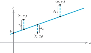
It sometimes happens that the theory behind an experiment indicates that the experimental data should lie approximately along a straight line of the form $y = mx +b$. The actual results, of course, never match the theory exactly. We are then faced with the problem of finding the straight line that best fits some set of experimental data $(x_1,y_1),\ldots,$ $(x_n,y_n)$ as in Figure 3.28. If we guess at a straight line $y = mx +b$ to fit the data, each point will deviate vertically from the line by an amount $d_i = y_i - (mx_i + b)$.

We would like to choose $m$ and $b$ in such a way as to make the total effect of these deviations as small as possible. However, because some are negative and some positive, we could get a lot of cancellations and still have a pretty bad fit. This leads us to suspect that a better measure of the total error might be the sum of the squares of these deviations. Thus, we are led to the problem of finding the $m$ and $b$ that minimize the function \[ s = f(m,b)= d_1^2 + d^2_2 + \cdots + d_n^2 = \sum_{i=1}^n\,(y_i - mx_i - b)^2, \] where $x_1,\ldots,x_n$ and $y_1,\ldots,y_n$ are the given data.

Figure 3.28: The method of least squares tries to find a straight line that best approximates a set of data.

Question 3.195

For each set of three data points, plot the points, write down the function $f(m,b)$ from the preceding equation, find $m$ and $b$ to give the best straight-line fit according to the method of least squares, and plot the straight line.

(a) $\begin{array}[t]{c} (x_1,y_1) = (1,1)\\ (x_2,y_2) = (2,3) \\ (x_3,y_3) = (4,3) \end{array}$
(b) $\begin{array}[t]{c} (x_1,y_1) = (0,0)\\ (x_2,y_2) = (1,2)\\ (x_3,y_3) = (2,3) \end{array}$

Question 3.196

Show that if only two data points $(x_1,y_1)$ and $(x_2,y_2)$ are given, this method produces the line through $(x_1,y_1)$ and $(x_2,y_2)$.

Question 3.197

Show that the equations for a critical point, $\partial s/\partial b =0$ and $\partial s /\partial m =0$, are equivalent to \[ m\bigg(\sum x_i\bigg)+ nb = \bigg(\sum y_i\bigg) \] and \[ m\bigg(\sum x_i^2\bigg)+ b\bigg(\sum x_i\bigg) = \bigg(\sum x_iy_i\bigg), \] where all the sums run from $i=1$ to $i=n$.

Question 3.198

If $y=mx +b$ is the best-fitting straight line to the data points $(x_1,y_1),\ldots,(x_n,y_n)$ according to the least-square method, show that \[ \sum_{i=1}^n\, (y_i - mx_i - b) =0; \] that is, the positive and negative deviations cancel (see Exercise 42).

215

Question 3.199

Use the second-derivative test to show that the critical point of $f$ is a minimum.

Question 3.200

Use the method of least squares to find the straight line that best fits the points $(0,1), (1,3),$ $(2,2), (3,4)$, and $(4,5)$. Plot the points and line.footnote #

Question 3.201

The partial differential equation \[ \frac{\partial^4 u}{\partial x^4} =-\frac{1}{c^2}\frac{\partial^2 u}{\partial t^2}, \] where $c$ is a constant, comes up in the study of deflections of a thin beam. Show that \[ u(x, t)=\sin(\lambda \pi x) \cos(\lambda^2 \pi^2 ct) \] is a solution for any choice of the parameter $\lambda$.

Question 3.202

The Kortweg–DeVries equation \[ \frac{\partial u}{\partial t} +u\frac{\partial u}{\partial x} +\frac{\partial^3 u}{\partial x^3} =0 \] arises in modeling shallow water waves (called $\textbf{solitons}$). Show that \[ u(x, t)=12a^2 \hbox{sech}^2(ax-4a^3t) \] is a solution to the Kortweg–DeVries equation (see the Internet supplement).

Question 3.203

The heat-conduction equation in two space dimensions is \[ k(u_{xx}+u_{yy})=u_t. \] Assuming that $u(x, y, t)=X(x)Y(y)T(t)$, find ordinary differential equations satisfied by $X(x), Y(y)$, and $T(t)$.

Question 3.204

The heat conduction equation in two space dimensions may be expressed in terms of polar coordinates as \[ k\Big(u_{rr}+ \frac{1}{r}u_r+ \frac{1}{r^2}u_{\theta \theta}\Big) =u_t. \] Assuming that $u(r, \theta, t)=R(r)\Theta(\theta)T(t)$, find ordinary differential equations satisfied by $R(r), \Theta(\theta)$, and $T(t)$.

216

¹Recall that integration by parts (the product rule for the derivative read backward) reads as: \[ \int_a^b u\,dv=uv|_a^b -\int_a^b v\,du. \] Here we choose $u=f'(\tau )$ and $v=x_{0}+h- \tau$.

²For the statement of the theorem as given here, $f$ actually needs only to be of class $C^2$, but for a convenient form of the remainder we assume $f$ is of class $C^3$.

³Proof If $g=0$, the result is clear, so we can suppose $g\neq 0$; thus, we can assume $\int_a^b g(t) \,{\it dt} > 0$. Let $M$ and $m$ be the maximum and minimum values of $h$, achieved at $t_M$ and $t_m$, respectively. Because $g(t) \ge 0$, \[ m \int_a^b g(t) \,{\it dt} \le \int_a^b h(t) g(t) \,{\it dt} \le M \int_a^b g(t) \,{\it dt}. \] Thus, $\big(\int_a^bh(t)g(t) \,{\it dt}\big)\big/\big(\int_a^bg(t) \,{\it dt}\big)$ lies between $m =h(t_m)$ and $M=h(t_M)$ and therefore, by the intermediate-value theorem, equals $h(c)$ for some intermediate $c$.

⁴The term “saddle point” is sometimes not used this generally; we shall discuss saddle points further in the subsequent development.

⁵Recall the proof from one-variable calculus: Because $g(0)$ is a local maximum, $g(t) \le g(0)$ for small $t > 0$, so $g(t) - g(0) \le 0$, and hence $g'(0) = {{\rm limit}_{t\to 0^+}}\,(g(t) - g(0))/t\le 0$, where ${{\rm limit}_{t\to 0^+}}$ means the limit as $t \to 0$, $t > 0$. For small $t < 0$, we similarly have $g'(0) = {{\rm limit}_{t\to 0^-}}\,(g(t) - g(0))/t \ge 0$. Therefore, $g'(0) =0$.

⁶Here we are using, without proof, a theorem analogous to a theorem in calculus that states that every continuous function on an interval $[a,b]$ achieves a maximum and a minimum; see Theorem 7.

⁷This is proved in, for example, K. Hoffman and R. Kunze, Linear Algebra, Prentice Hall, Englewood Cliffs, N.J., 1961, pp. 249–251. For students with sufficient background in linear algebra, it should be noted that $B$ is positive-definite when all of its eigenvalues (which are necessarily real, because $B$ is symmetric) are positive.

⁸This interesting phenomenon was first pointed out by the famous mathematician Giuseppe Peano (1858–1932). Another curious “pathology” is given in Exercise 41.

⁹In these examples, ${\nabla} g({\bf x}_0)\neq {\bf 0}$ on the surface $S$, as required by the Lagrange multiplier theorem. If ${\nabla}\! g({\bf x}_0)$ were zero for some ${\bf x}_0$ on $S$, then it would have to be included among the possible extrema.

¹⁰Dorothy L. Sayers, Have His Carcase, Chapter 31: The Evidence of the Haberdasher’s Assistant, New York, Avon Books, 1968, p. 312.

¹¹As with the hypothesis ${\nabla}\! g({\bf x}_0) \ne {\bf 0}$ in the Lagrange multiplier theorem, here we must assume that the vectors ${\nabla} g_1({\bf x}_0),\ldots, {\nabla} g_k({\bf x}_0)$ are linearly independent; that is, each $\nabla {g_i} ({\bf x}_0)$ is not a linear combination of the other $\nabla {g_j} ({\bf x}_0), j \,{\neq}\, i$.

¹²The matrix of coefficients of the equations cannot have an inverse, because this would imply that the solution is zero. Recall that a matrix that does not have an inverse has determinant zero.

¹³For a detailed discussion, see C. Caratheodory, Calculus of Variations and Partial Differential Equations, Holden-Day, San Francisco, 1965; Y. Murata, Mathematics for Stability and Optimization of Economic Systems, Academic Press, New York, 1977, pp. 263–271; or D. Spring, Am. Math. Mon. 92 (1985): 631–643.

¹⁴For three different proofs of the general case, consult: (a) E. Goursat, A Course in Mathematical Analysis, I, Dover, New York, 1959, p. 45. (This proof derives the general theorem by successive application of Theorem 11.) (b) T. M. Apostol, Mathematical Analysis, 2d ed., Addison-Wesley, Reading, Mass., 1974. (c) J. E. Marsden and M. Hoffman, Elementary Classical Analysis, 2d ed., Freeman, New York, 1993. Of these sources, the last two use more sophisticated ideas that are usually not covered until a junior-level course in analysis. The first, however, is easily understood by the reader who has some knowledge of linear algebra.

¹⁵For students who have had linear algebra: The condition $\Delta\neq 0$ has a simple interpretation in the case that $F$ is linear; namely, $\Delta\neq 0$ is equivalent to the rank of $F$ being equal to $m$, which in turn is equivalent to the fact that the solution space of $F=0$ is m-dimensional.

¹⁶The method of least squares may be varied and generalized in a number of ways. The basic idea can be applied to equations of more complicated curves than the straight line. For example, this might be done to find the parabola that best fits a given set of data points. These ideas also formed part of the basis for the development of the science of cybernetics by Norbert Wiener. Another version of the data is the following problem of least-square approximation: Given a function $f$ defined and integrable on an interval $[a,b]$, find a polynomial $P$ of degree ${\leq} n$ such that the mean square error \[ \int^b_a {\mid} f(x) - P(x) |^2 \,dx \] is as small as possible.